


The TikZ calc library enables you to build elaborate geometrical figures. More precisely, this library produces objets, mainly points, from primitive ones. Primitives objects are to be defined by their coordinates (cartesians or polar) but a wise rule is to use as few computations on the coordinates as possible. Here comes the calc library and we propose on this page to describe some simple applications of this powerful tool. We will limit ourselves to affine constructions and to figures containing essentially points and lines.
The calc library is invoked, in the preamble, by the command \usetikzlibrary{calc}.
In affine geometry, we are essentially concerned with parallelism and ratio of lengths, the length itself has no meaning in affine geometry. Vector equality is also a great concern. So, with just a few tools, we should be able to build about any plane affine construction. Of course, we’ll have now and then to build the intersections of lines.
The length ratio
Build the point P such that AP = λ·AB . P is given by \coordinate (P) at ($(A)!λ!(B)$);
The midpoint M of [AB] is then \coordinate (M) at ($(A)!0.5!(B)$); The symmetric S of A with respect to B is \coordinate (S) at ($(A)!2!(B)$); or \coordinate (S) at ($(B)!-1!(A)$);
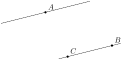
If you want to draw the line AB a bit further than points A and B, you’ll type
\begin{tikzpicture}
  \coordinate (A) at (-1,-1);
  \coordinate (B) at (1,0);
  \coordinate (A') at ($(A)!-0.3!(B)$);
  \coordinate (B') at ($(A)!1.3!(B)$);
  \draw (A')--(B');
  \fill (A) circle (0.5mm) node[above]{$A$};
  \fill (B) circle (0.5mm) node[below]{$B$};
\end{tikzpicture}
As this is often used, it is a good idea to make a macro out of it. Something like this:
\newcommand{\SmartLine}[2]{
  \coordinate (ATemp) at ($(#1)!-0.2!(#2)$);
  \coordinate (BTemp) at ($(#1)!1.2!(#2)$);
  \draw (ATemp)--(BTemp);
}
Or this
\newcommand{\CleverLine}[4]{
  \coordinate (ATemp) at ($(#1)!{-#3}!(#2)$);
  \coordinate (BTemp) at ($(#1)!{1+#4}!(#2)$);
  \draw (ATemp)--(BTemp);
}
Parameters #3 and #4 determine (in %), the extent to wich the line is prolonged in both direction.
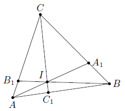
An easy construction is the one illustrating Ceva’s theorem:
AC1/C1B=BA1/A1C=CB1/B1A
\begin{tikzpicture}
  \coordinate[label=below:$A$] (A) at (-1,0);
  \coordinate[label=right:$B$] (B) at (2.5,0.5);
  \coordinate[label=above:$C$] (C) at (0,3);
  \coordinate[label=right:$A_1$] (A1) at ($(B)!0.3!(C)$);
  \coordinate[label=left:$B_1$] (B1) at ($(C)!0.8!(A)$);
  \coordinate[label=above left:$I$]
    (I) at (intersection of A--A1 and B--B1);
  \coordinate[label=below:$C_1$]
    (C1) at (intersection of C--I and A--B);
  \draw (A)--(B)--(C)--cycle;
  \draw (A)--(A1) (B)--(B1) (C)--(C1);
  \foreach \p in {A,B,C,A1,B1,C1,I}
  \fill (\p) circle (0.5mm);
\end{tikzpicture}
The fourth point of a parallelogram and vector equality
Determine the point D such that AD = BC . Who would say “I’ll never need that!”? D is simply determined by the line of code: \coordinate (D) at ($(A)+(C)-(B)$);
\begin{tikzpicture}
  \coordinate (A) at (-1,1);
  \coordinate (B) at (1.5,-0.5);
  \coordinate (C) at (1,1);
  \coordinate (D) at ($(A)+(C)-(B)$);
  \draw (A)--(B)--(C)--(D)--cycle;
  \foreach \p in {A,B,C,D}
  \fill (\p) circle (0.5mm) node [above right]{$\p$};
\end{tikzpicture}
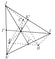
Here is an exercise that intensively uses this construction.
O is any point inside triangle ABC. I,J and K are such that OABI, OBCJ and OCAK are parallelograms. Prove that O is the center of gravity of triangle IJK.
\begin{tikzpicture}
  \coordinate[label=above:$A$] (A) at (-1,-1);
  \coordinate[label=below:$B$] (B) at (1.5,-1.2);
  \coordinate[label=left:$C$] (C) at (0.2,1);
  \coordinate[label=above:$O$] (O) at (0,0);
  \coordinate[label=above:$I$] (I) at ($(B)+(O)-(A)$);
  \coordinate[label=above:$J$] (J) at ($(C)+(O)-(B)$);
  \coordinate[label=below:$K$] (K) at ($(A)+(O)-(C)$);
  \coordinate[label=above:$K'$] (K') at ($(I)!0.5!(J)$);
  \coordinate[label=left:$I'$] (I') at ($(J)!0.5!(K)$);
  \coordinate[label=above:$J'$] (J') at ($(K)!0.5!(I)$);
  \draw[dashed] (O)--(A)--(B)--(I)--cycle;
  \draw[dashed] (O)--(B)--(C)--(J)--cycle;
  \draw[dashed] (O)--(C)--(A)--(K)--cycle;
  \draw (I)--(I') (J)--(J') (K)--(K');
  \draw[thick] (I)--(J)--(K)--cycle;
  \foreach \p in {A,B,C,I,J,K,O,I',J',K'}
  \fill (\p) circle (0.5mm);
\end{tikzpicture}
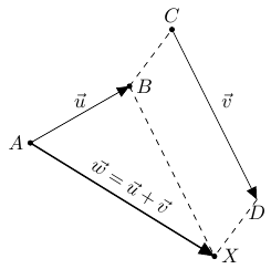
The sum of two vectors can be described by this:
\begin{tikzpicture}
  \coordinate[label=left:$A$] (A) at (-1,0);
  \coordinate[label=right:$B$]  (B) at (0.75,1);
  \coordinate[label=above:$C$]  (C) at (1.5,2);
  \coordinate[label=below:$D$]  (D) at (3,-1);
  \coordinate[label=right:$X$]  (X) at ($(B)+(D)-(C)$);
  \draw[->,>=triangle 45] (A)--(B)
    node[midway,above]{$\vec{u}$};
  \draw[->,>=triangle 45] (C)--(D)
    node[midway,above right]{$\vec{v}$};
  \draw[->,>=triangle 45,thick] (A)--(X)
    node[midway,sloped,above]
    {$\vec{w}=\vec{u}+\vec{v}$};
  \draw[dashed] (B)--(X) (B)--(C) (D)--(X);
  \foreach \p in {A,B,C,X} \fill (\p) circle (0.5mm);
\end{tikzpicture}
In this figure the arrow tips (the option ‘>=triangle 45’ of the \draw command) are obtained using the arrows library: \usetikzlibrary{arrows}.
As an exercise, we might propose this:
Given the parallelograms ABCD and A’B’C’D’ prove that the midpoints A”,B”, C”, D” of segments [AA’],[BB’],[CC’] and [DD’] are the vertices of a parallelogram (possibly degenerated).
The image should look like this:
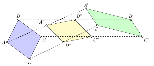
Remember that only points A,B,C and A’,B’,C’ are defined by their coordinates. The rest is determined by the calc library.
Parallelism
In order to draw the parallel to line BC through point A, you can define D such that AD = CB and D’ such that AD’=BC. Drawing line DD’ places A in the middle of segment [DD’].
\begin{tikzpicture}
  \coordinate (A) at (-2,1);
  \coordinate (B) at (1,-0.5);
  \coordinate (C) at (-1,-1);
  \coordinate (TempA) at ($(A)+(B)-(C)$);
  \coordinate (TempB) at ($(A)-(B)+(C)$);
  \draw (TempA)--(TempB);
  \CleverLine{B}{C}{.2}{.2}
  \foreach \p in {A,B,C}
    \fill (\p) circle (0.5mm) node [above right]{$\p$};
\end{tikzpicture}
A macro that draws the parallel to BC through point A could look like this:
\newcommand{\parallele}[5]{
  \coordinate (ATemp) at ($(#1)+(#3)-(#2)$);
  \coordinate (BTemp) at ($(#1)!{-#4}!(ATemp)$);
  \coordinate (CTemp) at ($(#1)!{1+#5}!(ATemp)$);
  \draw (BTemp)--(CTemp);
}
Points A, B and C correspond respectively to parameters #1, #2 and #3.
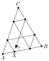
Thales Configuration
As an application of the intercept theorem (Thales’ theorem), we propose the following:
\begin{tikzpicture}
  \def\r{0.3}
  \coordinate[label=below:$A$] (A) at (-1,-1);
  \coordinate[label=right:$B$] (B) at (1.5,-0.5);
  \coordinate[label=above:$C$] (C) at (0,2);
  \coordinate[label=below:$X$] (X1) at ($(A)!\r!(B)$);
  \coordinate (X2) at ($(A)!\r!(C)$);
  \coordinate (X3) at ($(B)!\r!(C)$);
  \coordinate (X4) at ($(B)!\r!(A)$);
  \coordinate (X5) at ($(C)!\r!(A)$);
  \coordinate (X6) at ($(C)!\r!(B)$);
  \coordinate (P) at ($(X6)!0.9!(X1)$);
  \draw (A)--(B)--(C)--cycle;
  \draw[->,>=triangle 45]
    (X1)--(X2)--(X3)--(X4)--(X5)--(X6)--(P)
    node[right]{?};
  \foreach \p in {A,B,C,X1,X2,X3,X4,X5,X6}
    \fill (\p) circle (0.6mm);
\end{tikzpicture}
Starting from point X and following a path each time parallel to one side of triangle ABC, do we necessarily return to point X?
The parabola as envelope
To close this short presentation we propose a more elaborate construction.
On one arm of an angle the arbitrary segment e and, on the other, the segment f are marked off n times in succession from the vertex of the angle, and the segment endpoints are numbered, beginning from the vertex 0, 1, 2, …, n and n, n-1, …, 2, 1, 0 respectively.
Prove that the lines joining the points with the same number envelop a parabola.
A proof can be found, for example, in “100 Great Problems of Elementary Mathématics, Their History and Solution” by Heinrich Dörrie (Dover, 1958).
This is the kind of construction all of us have done, with paper and pencil, sometime when we were young in a class room. It is relatively easy to realize with the calc library and without any analytical geometry. Of course, as this is a repetitive task, well need some loop instruction (Tikz provides a very efficient loop structure : the \foreach instruction).
\begin{tikzpicture}[scale=0.4]
  \def\n{20} % nb. subdivisions OA and OB
  \def\m{8}  % nb. of tangents outside [OA], [OB]
  \def\la{10}% distance OA
  \def\lb{10}% dist. OB
  \def\a{-10}% angle OA
  \def\b{75}% angle OB
  \coordinate (O) at (0,0);
  \coordinate (A) at (\a:\la);
  \coordinate (B) at (\b:\lb);
  \draw[thick] ($(O)!2.5!(B)$)--($(B)!1.5!(O)$);
  \draw[thick] ($(O)!2.5!(A)$)--($(A)!1.5!(O)$);
  \foreach \i in {1,...,\n}{
    \draw[red] ($(O)!{\i/\n}!(A)$)--($(O)!{(1-\i/\n+1/\n}!(B)$);
  }
  \foreach \i in {1,...,\m}{
    \coordinate (X) at ($(O)!{1+\i/\n}!(A)$);
    \coordinate (Y) at ($(O)!{-\i/\n}!(B)$);
    \draw[blue] ($(X)!-0.8!(Y)$)--(Y);
    \coordinate (X) at ($(O)!{1+\i/\n}!(B)$);
    \coordinate (Y) at ($(O)!{-\i/\n}!(A)$);
    \draw[green] ($(X)!-0.8!(Y)$)--(Y);
  }
  \fill (A) circle (2pt)node[above]{$A$};
  \fill (B) circle (2pt)node[right]{$B$};
\end{tikzpicture}
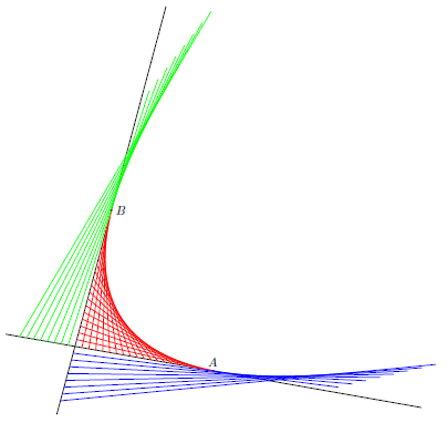
Drawing the initial lines (the red ones) won’t convince many of us that the envelope is indeed an arc of a parabola, it could be any hyperbolic segment for example. Fortunately, the construction can be completed with the blue and the green lines of the figure that are drawn in the same way as the red lines. The picture is then pedagogically much more convincing even if a rigourous proof has still to be delivered.