


The start
Let’s see, what would I be talking about that’s related to graphics? Well – almost everything I do, TeXnically speaking, is somehow related to chemistry. And in chemistry you have all kinds of graphics: potential energy curves, Haegg-diagrams, molecular orbital diagrams and of course all the sceletal formulas and reaction schemes common in (not only) organic chemistry.
The standard diagrams are not too complicated but are maybe worth an article in my blog. Molecular orbital diagrams are easily done with the package »MOdiagram«. So what’s left? Sceletal formulas? They’re easy if you glanced in the documentation of »ChemFig«. Well – most of them, anyway.
What about reaction schemes? Ever created one with LaTeX? No? Then it’s time! And »ChemFig« has just the tools for this.
»ChemFig« and reaction schemes
A note before I start: all the examples later use the packages chemfig and chemmacros and should run with a preamble like follows and an up to date TeX distribution.
\usepackage[T1]{fontenc}
\usepackage[utf8]{inputenc}
\usepackage{chemfig,chemmacros}

\chemsetup[chemformula]{format=\sffamily}
\renewcommand*\printatom[1]{\ensuremath{\mathsf{#1}}}
\setatomsep{2em}
\setdoublesep{.6ex}
\setbondstyle{semithick}
An easy start
In my experience the scheming mechanisms of »ChemFig« are still rather unknown although they’re also not too complicated once you’ve mastered the one command:
\arrow(from--to){type[above][below][shift]}[angle,length,tikz]
The last option reminds us: »ChemFig« uses TikZ to draw molecules and schemes. I will also make use of TikZ but I won’t explicitly explain TikZ code. This is about »ChemFig« after all. Back to \arrow. All of its arguments are optional. So the basic use is very intuitive again:
\begin{center}
 \schemestart
  \chemfig{-[:30](-[2])-[:-30]OH}
  \arrow
  \chemfig{-[:30](-[2])=^[:-30]O}
 \schemestop
\end{center}
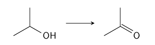
Creating something like this poses not a big challenge, then:
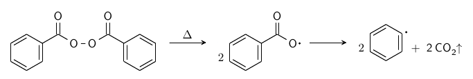
\begin{center}\small\setatomsep{1.5em}
 \schemestart
 \chemfig{*6(=-=(-(=[2]O)-[::-60]O-[0]O-[::30](=[2]O)-[::-60]*6(=-=-=-))-=-)}
  \arrow{->[$\Delta$]}
  2 \chemfig{*6(=-=(-(=[2]O)-[::-60]\lewis{0.,O})-=-)}
  \arrow
  2 \chemfig{*6(=-=(-[,.15,,,draw=none]\lewis{0.,})-=-)}\+\ch{2 CO2 ^}
 \schemestop
\end{center}
Get more sophisticated
But what if the scheme gets bigger, maybe has branches or something? Or is educational like this one:
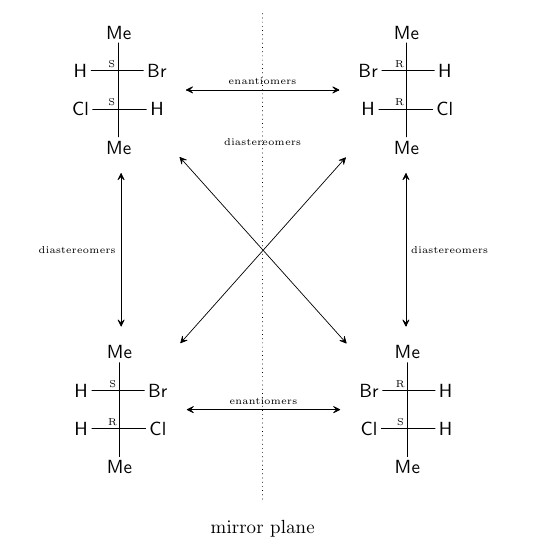
The code looks as follows. Let’s decrypt it step by step:
\begin{center}%\schemedebug{true}
\makeatletter
 \definearrow{0}{..}{\draw[dotted] (\CF@arrow@start@node)--(\CF@arrow@end@node);}
\makeatother
\definesubmol{\conf}{-[:135,.25,,,draw=none]}
\schemestart
 \chemfig{[6]Me-(!\conf{\text{\tiny S}})(-[0]Br)(-[4]H)-(!\conf{\text{\tiny S}})(-[0]H)(-[4]Cl)-Me}
 \arrow(a--b){<->[\tiny enantiomers]}[,2,line width=.4pt]
 \chemfig{[6]Me-(!\conf{\text{\tiny R}})(-[0]H)(-[4]Br)-(!\conf{\text{\tiny R}})(-[0]Cl)(-[4]H)-Me}
 \arrow{<->[*0\tiny diastereomers]}[-90,2,line width=.4pt]
 \chemfig{[6]Me-(!\conf{\text{\tiny R}})(-[0]H)(-[4]Br)-(!\conf{\text{\tiny S}})(-[0]H)(-[4]Cl)-Me}
 \arrow(c--d){<->[\tiny enantiomers]}[180,2,line width=.4pt]
 \chemfig{[6]Me-(!\conf{\text{\tiny S}})(-[0]Br)(-[4]H)-(!\conf{\text{\tiny R}})(-[0]Cl)(-[4]H)-Me}
 \arrow{<->[*0\tiny diastereomers]}[90,2,line width=.4pt]
 \arrow(@a--@c){<->}[,,line width=.4pt]
 \arrow(@b--@d){<->}[,,line width=.4pt]
 \arrow(@a--xx){0}[,1]{}\arrow{0}[-90,.5] \tiny diastereomers
 \arrow(@xx--){0}[90,1]{}\arrow{..}[-90,5.5] mirror plane
\schemestop
\end{center}
We’ll ignore the first few lines for the moment and we’ll also ignore the formulas. Then we have this:
\schemestart
 upper left compound
 \arrow(a--b){<->[\tiny enantiomers]}[,2,line width=.4pt]
The first argument (a--b) names the node of the “upper left compound” a and the one following the arrow b. We’ll see later what’s that for. The second argument {<->[\tiny enantiomers]} chooses the type <-> and a label that should be written above the arrow. The third argument [,2,line width=.4pt] multiplies the length of the arrow by 2 and adds a TikZ style for the line width.
 upper right compound
 \arrow{<->[*0\tiny diastereomers]}[-90,2,line width=.4pt]
This is almost the same. There are two differences, though: 1) the last argument [-90,2,line width=.4pt] tells the arrow to go down (angle = -90). 2) The optional argument of the arrow type begins with *0 which means that the label should be rotated by 0 degrees. Otherwise it would be rotated together with the arrow.
There’s nothing new in the next four lines:
 lower right compound
 \arrow(c--d){<->[\tiny enantiomers]}[180,2,line width=.4pt]
 lower left compound
 \arrow{<->[*0\tiny diastereomers]}[90,2,line width=.4pt]
But then it gets more interesting:
 \arrow(@a--@c){<->}[,,line width=.4pt]
 \arrow(@b--@d){<->}[,,line width=.4pt]
These are the diagonal arrows. Now we can profit from the fact that we named the compounds. (@a--@c) connects the upper left with the lower right compound, for example. You can see that you use the names you’ve given with an @ before it. »ChemFig« names the compounds itself, by the way. If you don’t choose names, they’re named c1, c2 and so forth. To help you not to lose track you can visualize the names, the nodes the compounds are in and a few additional information by saying \schemedebug{true}.
In the last lines we do some invisible things. The arrow type 0 is an invisible arrow. We use it to add an inscription above the crossed arrows in the center of the scheme: go left by 1 arrow length from compound a, name the empty compound xx, then go down by half an arrow length:
 \arrow(@a--xx){0}[,1]{}\arrow{0}[-90,.5] \tiny diastereomers
 \arrow(@xx--){0}[90,1]{}\arrow{..}[-90,5.5] mirror plane
\schemestop
In line 18 we go up from the empty compound xx and use the arrow type we’ve defined in lines 2–4 to draw the dotted line indicating the mirror plane. Yes, that’s true: you can define your own arrow types. In this case it is a fairly simple one:
\makeatletter
 \definearrow{0}{..}{\draw[dotted] (\CF@arrow@start@node)--(\CF@arrow@end@node);}
\makeatother
An arrow type with 0 optional arguments whose symbol is .. and simply draws a dotted line from the start to the end \draw[dotted] (\CF@arrow@start@node)--(\CF@arrow@end@node);.
Get colorful
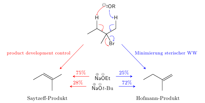
Want more? Let’s get educational one more time (that’s what I do…) and add some fancy colors (I’m sorry this is in German, but that’s my native language and frankly I’ve been to lazy to translate it):
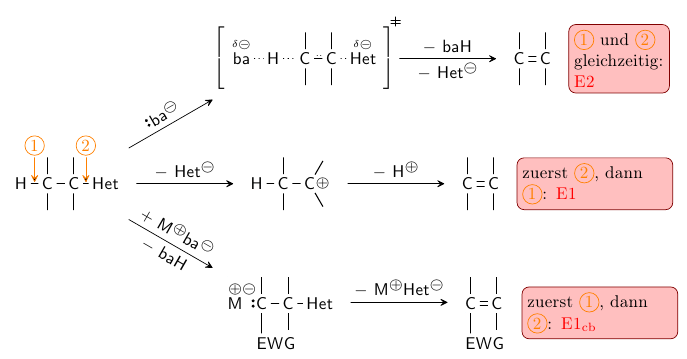
Now, there’s some work to do before we can start the actual scheme:
\begin{center}
 \small\chemsetup[option]{circled=all}
 % chemfig settings:
 \renewcommand*\printatom[1]{\ensuremath{\mathsf{#1}}}
 \setdoublesep{.6ex}
 \setatomsep{1.5em}
 \setarrowdefault{,1.5}
 % shortcuts for two circled numbers:
 \def\eins{\tikz{\node[orange,draw=orange,circle,inner sep=1pt,text width=1.2ex]{1};}}
 \def\zwei{\tikz{\node[orange,draw=orange,circle,inner sep=1pt,text width=1.2ex]{2};}}
 % we need to define a decoration that we can use for a bond type between
 % single and double, with some delocalized electrons; this is TikZ/pgf,
 % actually:
 \usetikzlibrary{matrix,decorations.pathmorphing}
 \pgfdeclaredecoration{ddbond}{initial}{%
   \state{initial}[width=2pt]{%
     \pgfpathlineto{\pgfpoint{2pt}{0pt}}%
     \pgfpathmoveto{\pgfpoint{1.5pt}{2pt}}%
     \pgfpathlineto{\pgfpoint{2pt}{2pt}}%
     \pgfpathmoveto{\pgfpoint{2pt}{0pt}}%
   }%
   \state{final}{%
     \pgfpathlineto{\pgfpointdecoratedpathlast}%
   }%
 }
 % finally some styles:
 \tikzset{
   info/.style   ={draw=red!50!black,fill=red!25,rounded corners,inner sep=3pt,font=\small},
   Uez/.style    ={left delimiter={[},right delimiter={]},inner sep=3pt},
   lddbond/.style={decorate,decoration=ddbond}}
Since I’m not talking about TikZ here I won’t go into detail of this code, I simply added a few comments. You’ll have to live with this for now. Here’s the code for the scheme:
 \schemestart
 \chemfig{H-[@{b1}]C(-[2])(-[6])-C(-[2])(-[6])-[@{b2},1.2]Het}
  % Label an die Bindungen:
  \arrow(@b1--[yshift=-.9em]){<-}[90,.5,draw=orange,shorten <=-.9em]\eins
  \arrow(@b2--[yshift=-.9em]){<-}[90,.5,draw=orange,shorten <=-.9em]\zwei
  % 1.)
  \arrow(@c1--.south west[Uez]){->[\lewis{4:,ba\mch}]}[30]
  \chemfig{\chemabove{ba}{\delm}-[,1.2,,,dotted]H-[,1.2,,,dotted]C(-[2])(-[6])-[,,,,lddbond]C(-[2])(-[6])-[,1.2,,,dotted]\chemabove{Het}{\delm}}
  \arrow{->[$-$ \ch{baH}][$-$ \ch{Het-}]}
  \chemfig{C(-[2])(-[6])=C(-[2])-[6]}
  \arrow(--[info,text width=1.8cm]){0}[,.2]
  {\eins\ und \zwei\ gleichzeitig: \textcolor{red}{\mech[e2]}}
  \arrow(@c4.north east--){0}[20,.1]\transitionstatesymbol
  % 2.)
  \arrow(@c1--){->[$-$ \ch{Het-}]}
  \chemfig{H-C(-[2])(-[6])-C(-[:60])(-[:-60])-[,.5,,,draw=none]\scrp}
  \arrow{->[$-$ \Hpl]}
  \chemfig{C(-[2])(-[6])=C(-[2])-[6]}
  \arrow(--[info,text width=2.9cm]){0}[,.2]
  {zuerst \zwei, dann \eins: \textcolor{red}{\mech[e1]}}
  % 3.)
  \arrow(@c1--.north west){->[$+$ \ch{M^+ba-}][$-$ \ch{baH}]}[-30]
  \chemfig{\chemabove{M}{\scrp}-[,,,,draw=none]\chemabove{\lewis{4:,C}}{\hspace{-.5cm}\scrm}(-[2])(-[6,1.5]E|WG)-C(-[2])(-[6])-[,1.2]Het}
  \arrow{->[$-$ \ch{M^+Het-}][][6pt]}
  \chemfig{C(-[2])(-[6,1.5]E|WG)=C(-[2])-[6]}
  \arrow(--[info,text width=2.9cm]){0}[,.2]
  {zuerst \eins, dann \zwei: \textcolor{red}{\mech[cb]}}
 \schemestop
\end{center}
You’ll notice some unfamiliar macros in there, probably, like \delm or \mech. They’re from the package »chemmacros« and of no further interest here. Maybe something for another blog post.
Let’s pick some lines that tell us something new:
  \chemfig{H-[@{b1}]C(-[2])(-[6])-C(-[2])(-[6])-[@{b2},1.2]Het}
  % Label an die Bindungen:
  \arrow(@b1--[yshift=-.9em]){<-}[90,.5,draw=orange,shorten <=-.9em]\eins
You maybe know that you can name nodes inside a formula created with \chemfig. This is done by adding @{name} at the appropriate place in the formula. We use this to add an arrow with a description to a bond. The arrow starts at the denoted bond b1 \arrow(@b1--[yshift=-.9em]){<-}. The node where it is ending is shifted a little bit down. That's new: you can add TikZ options to the nodes where an arrow starts or ends with an optional argument.
\arrow(name.anchor[tikz]--name.anchor[tikz])
The scheme uses this possibility quite frequently, for example here:
\arrow(@c1--.south west[Uez]){->[\lewis{4:,ba\mch}]}[30]
This means: start from compound c1, use an angle of 30 degrees and end at the south west corner of the following compound. Use the TikZ style Uez here.
The end
I could add loads and loads of other examples but I think the basics should be clear now. You have seen that »ChemFig's« \arrow is a powerful thing and one can create nice schemes. From my personal experience I want to add: if you're more or less familiar with TikZ and have learned the syntax of the \arrow creating these themes doesn't really take much time and also is fun!
A teaser: rebuilt the one below with »ChemFig« and »chemmacros«! And most importantly: have fun!
Happy TeXing!