


When I started working on my thesis dissertation using LaTeX, I discovered the TikZ package for drawing vector-based figures. I needed a way to easily draw three-dimensional figures, and so I put together a few handy tools in the tikz-3dplot package. This package builds on TikZ, providing an easy way to rotate the perspective when drawing three-dimensional shapes using basic shapes in a tikzpicture environment.
Let’s explore some examples of what tikz-3dplot can do.
– A contribution to the LaTeX and Graphics contest – This article is available for reading and for download in pdf format –
The Basics
Let’s draw a cube, with side length of 2. To help illustrate the comparison, we’ll draw a grid in the x–y plane, and also show the x, y, and z axes.
\begin{tikzpicture}
		[cube/.style={very thick,black},
			grid/.style={very thin,gray},
			axis/.style={->,blue,thick}]

	%draw a grid in the x-y plane
	\foreach \x in {-0.5,0,...,2.5}
		\foreach \y in {-0.5,0,...,2.5}
		{
			\draw[grid] (\x,-0.5) -- (\x,2.5);
			\draw[grid] (-0.5,\y) -- (2.5,\y);
		}

	%draw the axes
	\draw[axis] (0,0,0) -- (3,0,0) node[anchor=west]{$x$};
	\draw[axis] (0,0,0) -- (0,3,0) node[anchor=west]{$y$};
	\draw[axis] (0,0,0) -- (0,0,3) node[anchor=west]{$z$};

	%draw the top and bottom of the cube
	\draw[cube] (0,0,0) -- (0,2,0) -- (2,2,0) -- (2,0,0) -- cycle;
	\draw[cube] (0,0,2) -- (0,2,2) -- (2,2,2) -- (2,0,2) -- cycle;

	%draw the edges of the cube
	\draw[cube] (0,0,0) -- (0,0,2);
	\draw[cube] (0,2,0) -- (0,2,2);
	\draw[cube] (2,0,0) -- (2,0,2);
	\draw[cube] (2,2,0) -- (2,2,2);

\end{tikzpicture}
\tdplotsetmaincoords{60}{125}
\begin{tikzpicture}
		[tdplot_main_coords,
			cube/.style={very thick,black},
			grid/.style={very thin,gray},
			axis/.style={->,blue,thick}]

	%draw a grid in the x-y plane
	\foreach \x in {-0.5,0,...,2.5}
		\foreach \y in {-0.5,0,...,2.5}
		{
			\draw[grid] (\x,-0.5) -- (\x,2.5);
			\draw[grid] (-0.5,\y) -- (2.5,\y);
		}


	%draw the axes
	\draw[axis] (0,0,0) -- (3,0,0) node[anchor=west]{$x$};
	\draw[axis] (0,0,0) -- (0,3,0) node[anchor=west]{$y$};
	\draw[axis] (0,0,0) -- (0,0,3) node[anchor=west]{$z$};

	%draw the top and bottom of the cube
	\draw[cube] (0,0,0) -- (0,2,0) -- (2,2,0) -- (2,0,0) -- cycle;
	\draw[cube] (0,0,2) -- (0,2,2) -- (2,2,2) -- (2,0,2) -- cycle;

	%draw the edges of the cube
	\draw[cube] (0,0,0) -- (0,0,2);
	\draw[cube] (0,2,0) -- (0,2,2);
	\draw[cube] (2,0,0) -- (2,0,2);
	\draw[cube] (2,2,0) -- (2,2,2);

\end{tikzpicture}
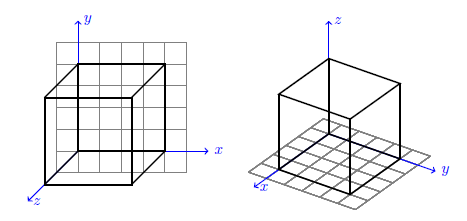
In the default configuration, shown on the left, the xy plane lies in the same plane as the page. The z-axis extends down and to the left, giving the illusion of depth. This is a useful representation of a three-dimensional space as is, but gives little in the range of customization.
The tikz-3dplot package can redefine the perspective for viewing this three-dimensional space. In the tikz-3dplot configuration, the z-axis points in the vertical direction, and the viewed perspective of the xy plane can be specified using the user-specified values θ and φ (in degrees). These angles define the direction from which the three-dimensional space is viewed, using the standard definition of the polar and azimuthal angles from polar coordinates.
To specify the display orientation, use the command \tdplotsetmaincoords{θ}{φ} before the tikzpicture environment, and include the tdplot_main_coords style within any drawing command. Alternatively, as seen in this example, you can include the tdplot_main_coords style within the global style settings of the tikzpicture environment.
As suggested by the name, tdplot_main_coords, I refer to this coordinate frame as the “main” coordinate frame. It provides the base through which you can perform all drawing operations. It may seem a bit restrictive that the z-axis of the main coordinate frame can only the vertical direction. If you wish to define a more general orientation, there is a second, “rotated” coordinate frame that can be specified relative to the orientation of the main coordinate frame. Let’s take a look at this cube example again, drawn in the rotated coordinate frame.
\tdplotsetmaincoords{60}{120}%
\tdplotsetrotatedcoords{0}{20}{0}%
\begin{tikzpicture}
		[tdplot_rotated_coords,
			cube/.style={very thick,black},
			grid/.style={very thin,gray},
			axis/.style={->,blue,thick},
			rotated axis/.style={->,purple,thick}]

	%draw a grid in the x-y plane
	\foreach \x in {-0.5,0,...,2.5}
		\foreach \y in {-0.5,0,...,2.5}
		{
			\draw[grid] (\x,-0.5) -- (\x,2.5);
			\draw[grid] (-0.5,\y) -- (2.5,\y);
		}

	%draw the main coordinate frame axes
	\draw[axis,tdplot_main_coords] (0,0,0) -- (3,0,0) node[anchor=west]{$x$};
	\draw[axis,tdplot_main_coords] (0,0,0) -- (0,3,0) node[anchor=north west]{$y$};
	\draw[axis,tdplot_main_coords] (0,0,0) -- (0,0,3) node[anchor=west]{$z$};


	%draw the rotated coordinate frame axes
	\draw[rotated axis] (0,0,0) -- (3,0,0) node[anchor=west]{$x'$};
	\draw[rotated axis] (0,0,0) -- (0,3,0) node[anchor=south west]{$y'$};
	\draw[rotated axis] (0,0,0) -- (0,0,3) node[anchor=west]{$z'$};

	%draw the top and bottom of the cube
	\draw[cube] (0,0,0) -- (0,2,0) -- (2,2,0) -- (2,0,0) -- cycle;
	\draw[cube] (0,0,2) -- (0,2,2) -- (2,2,2) -- (2,0,2) -- cycle;

	%draw the edges of the cube
	\draw[cube] (0,0,0) -- (0,0,2);
	\draw[cube] (0,2,0) -- (0,2,2);
	\draw[cube] (2,0,0) -- (2,0,2);
	\draw[cube] (2,2,0) -- (2,2,2);

\end{tikzpicture}
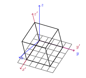
Here, I show the axes for both the main coordinate frame (xyz) and rotated coordinate frame (x‘y‘z‘). Using the command \tdplotsetrotatedcoords{θz}{θy}{θz}, the rotated coordinate frame is defined by taking the orientation of the main coordinate frame, and then performing the Euler angle rotations (θz, θy, θz) (in degrees) to define the rotated coordinate frame. The coordinate transformation for the rotated coordinate frame is stored in the tdplot_rotated_coords style. In this example, I simply rotated about the y-axis of the main coordinate frame.
Examples
Defining tdplot_main_coord and tdplot_rotated_coords is just the beginning. tikz-3dplot provides a bunch of handy tools to make it easier to work in a three-dimensional space.
Defining Coordinates
For example, the command \tdplotsetcoord{r}{θ}{φ} defines a coordinate using spherical coordinates r, θ, φ. More than that, this handy command also defines points that can be useful for projections on the axes and their shared planes. Consider the following example, where the coordinate (P) is defined in the three-dimensional space using spherical polar coordinates.
\tdplotsetmaincoords{60}{120}
\begin{tikzpicture}
	[scale=3,
		tdplot_main_coords,
		axis/.style={->,blue,thick},
		vector/.style={-stealth,red,very thick}]

	%standard tikz coordinate definition using x, y, z coords
	\coordinate (O) at (0,0,0);

	%tikz-3dplot coordinate definition using r, theta, phi coords
	\tdplotsetcoord{P}{.8}{55}{60}

	%draw axes
	\draw[axis] (0,0,0) -- (1,0,0) node[anchor=north east]{$x$};
	\draw[axis] (0,0,0) -- (0,1,0) node[anchor=north west]{$y$};
	\draw[axis] (0,0,0) -- (0,0,1) node[anchor=south]{$z$};

	%draw a vector from O to P
	\draw[vector] (O) -- (P);
\end{tikzpicture}
\tdplotsetmaincoords{60}{120}
\begin{tikzpicture}
	[scale=3,
		tdplot_main_coords,
		axis/.style={->,blue,thick},
		vector/.style={-stealth,red,very thick},
		vector guide/.style={dashed,red,thick}]

	%standard tikz coordinate definition using x, y, z coords
	\coordinate (O) at (0,0,0);

	%tikz-3dplot coordinate definition using r, theta, phi coords
	\tdplotsetcoord{P}{.8}{55}{60}

	%draw axes
	\draw[axis] (0,0,0) -- (1,0,0) node[anchor=north east]{$x$};
	\draw[axis] (0,0,0) -- (0,1,0) node[anchor=north west]{$y$};
	\draw[axis] (0,0,0) -- (0,0,1) node[anchor=south]{$z$};

	%draw a vector from O to P
	\draw[vector] (O) -- (P);

	%draw guide lines to components
	\draw[vector guide] (O) -- (Pxy);
	\draw[vector guide] (Pxy) -- (P);
\end{tikzpicture}
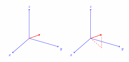
In the left diagram, it is hard to identify where the vector lies in the three-dimensional space. In the right diagram, I make use of the (automatically generated) projection coordinate (Pxy), which lies in the xy plane below (P), to illustrate the orientation of the vector.
Drawing Circles and Arcs
To draw a circle or arc, the \tdplotdrawarc command is provided. Here, you specify the center of the circle/arc, the radius, the start and end angles, and label notes. Here are a couple examples that use arcs and circles.
\tdplotsetmaincoords{60}{120}
\begin{tikzpicture}
	[scale=3,
		tdplot_main_coords,
		axis/.style={->,blue,thick},
		vector/.style={-stealth,red,very thick},
		vector guide/.style={dashed,red,thick},
		angle/.style={red,thick}]

	%standard tikz coordinate definition using x, y, z coords
	\coordinate (O) at (0,0,0);

	%tikz-3dplot coordinate definition using r, theta, phi coords
	\tdplotsetcoord{P}{.8}{55}{60}

	%draw axes
	\draw[axis] (0,0,0) -- (1,0,0) node[anchor=north east]{$x$};
	\draw[axis] (0,0,0) -- (0,1,0) node[anchor=north west]{$y$};
	\draw[axis] (0,0,0) -- (0,0,1) node[anchor=south]{$z$};

	%draw a vector from O to P
	\draw[vector] (O) -- (P);

	%draw guide lines to components
	\draw[vector guide] (O) -- (Pxy);
	\draw[vector guide] (Pxy) -- (P);

	%draw an arc illustrating the angle defining the orientation
	\tdplotdrawarc[angle]{(O)}{.35}{0}{60}{anchor=north}{$\phi$}

	%define the rotated coordinate frame to lie in the "theta plane"
	\tdplotsetthetaplanecoords{55}

	\tdplotdrawarc[tdplot_rotated_coords,angle]{(O)}{.35}{0}{55}
          {anchor=south west}{$\theta$}

\end{tikzpicture}
\tdplotsetmaincoords{55}{5}
\begin{tikzpicture}
	[scale=3,
		tdplot_main_coords,
		curve/.style={red,densely dotted,thick}]

	\coordinate (O) at (0,0,0);

	\foreach \angle in {-90,-75,...,90}
	{
		%calculate the sine and cosine of the angle
		\tdplotsinandcos{\sintheta}{\costheta}{\angle}%

		%define a point along the z-axis through which to draw
		%a circle in the xy-plane
		\coordinate (P) at (0,0,\sintheta);

		%draw the circle in the main frame
		\tdplotdrawarc[curve]{(P)}{\costheta}{0}{360}{}{}

		%define the rotated coordinate frame based on the angle
		\tdplotsetthetaplanecoords{\angle}

		%draw the circle in the rotated frame
		\tdplotdrawarc[curve,tdplot_rotated_coords]{(O)}{1}{0}{360}{}{}
	}

\end{tikzpicture}
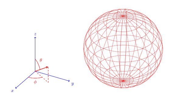
The left example is an extension of the vector example shown earlier. An arc was added in the xy plane to illustrate the azimuthal angle, φ, and another arc was added to illustrate the polar angle, θ. In the right example, a series of circles are drawn to represent longitudinal and latitudinal lines on a sphere.
To make these examples, a few useful helper functions are used. First, the \tdplotsetthetaplanecoords{φ} function gives a convenient way of placing rotated coordinate frame such that the x‘y‘ plane is lined up to draw the polar angle, θ. Second, the \tdplotsinandcos{\sintheta}{\costheta}{θ} command takes the specified angle, θ (in degrees), and stores the sine and cosine value of that angle in the macros \sintheta and \costheta. Note that you can use any name in place of \sintheta and \costheta for your convenience.
Drawing Surfaces
Drawing lines and curves can be great fun, but what if you wanted to represent a solid object with opaque surfaces? With proper planning and careful consideration of which surfaces are drawn first, you can render simple shapes.
\tdplotsetmaincoords{60}{125}
\begin{tikzpicture}
	[tdplot_main_coords,
		grid/.style={very thin,gray},
		axis/.style={->,blue,thick},
		cube/.style={opacity=.5,very thick,fill=red}]
	%draw a grid in the x-y plane
	\foreach \x in {-0.5,0,...,2.5}
		\foreach \y in {-0.5,0,...,2.5}
		{
			\draw[grid] (\x,-0.5) -- (\x,2.5);
			\draw[grid] (-0.5,\y) -- (2.5,\y);
		}

	%draw the axes
	\draw[axis] (0,0,0) -- (3,0,0) node[anchor=west]{$x$};
	\draw[axis] (0,0,0) -- (0,3,0) node[anchor=west]{$y$};
	\draw[axis] (0,0,0) -- (0,0,3) node[anchor=west]{$z$};

	%draw the bottom of the cube
	\draw[cube] (0,0,0) -- (0,2,0) -- (2,2,0) -- (2,0,0) -- cycle;

	%draw the back-right of the cube
	\draw[cube] (0,0,0) -- (0,2,0) -- (0,2,2) -- (0,0,2) -- cycle;

	%draw the back-left of the cube
	\draw[cube] (0,0,0) -- (2,0,0) -- (2,0,2) -- (0,0,2) -- cycle;


	%draw the front-right of the cube
	\draw[cube] (2,0,0) -- (2,2,0) -- (2,2,2) -- (2,0,2) -- cycle;

	%draw the front-left of the cube
	\draw[cube] (0,2,0) -- (2,2,0) -- (2,2,2) -- (0,2,2) -- cycle;

	%draw the top of the cube
	\draw[cube] (0,0,2) -- (0,2,2) -- (2,2,2) -- (2,0,2) -- cycle;

\end{tikzpicture}
\tdplotsetmaincoords{60}{125}
\begin{tikzpicture}[
		tdplot_main_coords,
		grid/.style={very thin,gray},
		axis/.style={->,blue,thick},
		cube/.style={very thick,fill=red},
		cube hidden/.style={very thick,dashed}]
	%draw a grid in the x-y plane
	\foreach \x in {-0.5,0,...,2.5}
		\foreach \y in {-0.5,0,...,2.5}
		{
			\draw[grid] (\x,-0.5) -- (\x,2.5);
			\draw[grid] (-0.5,\y) -- (2.5,\y);
		}

	%draw the axes
	\draw[axis] (0,0,0) -- (3,0,0) node[anchor=west]{$x$};
	\draw[axis] (0,0,0) -- (0,3,0) node[anchor=west]{$y$};
	\draw[axis] (0,0,0) -- (0,0,3) node[anchor=west]{$z$};

	%draw the front-right of the cube
	\draw[cube] (2,0,0) -- (2,2,0) -- (2,2,2) -- (2,0,2) -- cycle;

	%draw the front-left of the cube
	\draw[cube] (0,2,0) -- (2,2,0) -- (2,2,2) -- (0,2,2) -- cycle;

	%draw the top of the cube
	\draw[cube] (0,0,2) -- (0,2,2) -- (2,2,2) -- (2,0,2) -- cycle;

	%draw dashed lines to represent hidden edges
	\draw[cube hidden] (0,0,0) -- (2,0,0);
	\draw[cube hidden] (0,0,0) -- (0,2,0);
	\draw[cube hidden] (0,0,0) -- (0,0,2);

\end{tikzpicture}
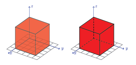
The left example uses fill color transparency to illustrate surfaces hidden behind others. Here, the covered and back edges of the cube are distinguished by having the fill for the front surfaces drawn over top. The right example has opaque front surfaces of the cube drawn first, and then the back edges are illustrated using dashed lines. In both situations, the order of drawing depends on the perspective. If you change the orientation of the coordinate frame, you will need to be careful about whether the drawing order needs to change. In the case with dashed lines, you may even need to reassign roles to the components of the object.
Another example of surface plots is the \tdplotsphericalsurfaceplot command. This command was developed to allow me to plot complex spherical harmonics, where the radius and hue of the surface is plotted as a function of the polar and azimuthal angles.
\tdplotsetmaincoords{70}{135}
\begin{tikzpicture}[scale=4,line join=bevel,tdplot_main_coords, fill opacity=.5]
	\pgfsetlinewidth{.2pt}
	\tdplotsphericalsurfaceplot[parametricfill]{72}{36}{sin(\tdplottheta)*cos(\tdplottheta)}{black}{\tdplotphi}%
		{\draw[color=black,thick,->] (0,0,0) -- (1,0,0) node[anchor=north east]{$x$};}%
		{\draw[color=black,thick,->] (0,0,0) -- (0,1,0) node[anchor=north west]{$y$};}%
		{\draw[color=black,thick,->] (0,0,0) -- (0,0,1) node[anchor=south]{$z$};}%
\end{tikzpicture}
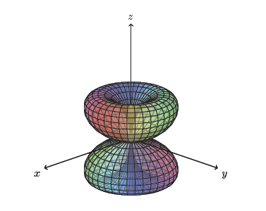
Here, I am plotting the function r = sin(θ)cos(θ), and using φ as the parameter to choose the surface fill hue. The instructions for \tdplotsphericalsurfaceplot define the angular step sizes, the function to plot, the line style, the fill style, and instructions for drawing axes. Unlike the manual surface plot examples shown earlier, the \tdplotsphericalsurfaceplot command does the work of determining how to appropriately draw the surface so that surfaces and edges drawn on the back side are appropriately rendered below those on the front. The only downside with this is that it takes some time to render, so you may want to look into externalizing these figures.
Limitations
When drawing shapes in tikz-3dplot, only simple shapes like line segments and arcs behave properly, whereas more involved shapes like rectangles and grids do not adhere to the sense of rotated coordinate system. Let’s look at the first example again, where we use the rectangle command to draw the top and bottom of the cube, rather than a series of line segments.
\begin{tikzpicture}
	%draw a grid in the x-y plane
	\foreach \x in {-0.5,0,...,2.5}
		\foreach \y in {-0.5,0,...,2.5}
		{
			\draw[gray,very thin] (\x,-0.5) -- (\x,2.5);
			\draw[gray,very thin] (-0.5,\y) -- (2.5,\y);
		}

	%draw the axes
	\draw[->] (0,0,0) -- (3,0,0) node[anchor=west]{$x$};
	\draw[->] (0,0,0) -- (0,3,0) node[anchor=west]{$y$};
	\draw[->] (0,0,0) -- (0,0,3) node[anchor=west]{$z$};

	%draw the top and bottom of the cube
	\draw[very thick] (0,0,0) rectangle (2,2,0);
	\draw[very thick] (0,0,2) rectangle (2,2,2);

	%draw the edges of the cube
	\draw[very thick] (0,0,0) -- (0,0,2);
	\draw[very thick] (0,2,0) -- (0,2,2);
	\draw[very thick] (2,0,0) -- (2,0,2);
	\draw[very thick] (2,2,0) -- (2,2,2);

\end{tikzpicture}
\tdplotsetmaincoords{60}{125}
\begin{tikzpicture}[tdplot_main_coords]
	%draw a grid in the x-y plane
	\foreach \x in {-0.5,0,...,2.5}
		\foreach \y in {-0.5,0,...,2.5}
		{
			\draw[gray,very thin] (\x,-0.5) -- (\x,2.5);
			\draw[gray,very thin] (-0.5,\y) -- (2.5,\y);
		}

	%draw the axes
	\draw[->] (0,0,0) -- (3,0,0) node[anchor=west]{$x$};
	\draw[->] (0,0,0) -- (0,3,0) node[anchor=west]{$y$};
	\draw[->] (0,0,0) -- (0,0,3) node[anchor=west]{$z$};

	%draw the top and bottom of the cube
	\draw[very thick] (0,0,0) rectangle (2,2,0);
	\draw[very thick] (0,0,2) rectangle (2,2,2);

	%draw the edges of the cube
	\draw[very thick] (0,0,0) -- (0,0,2);
	\draw[very thick] (0,2,0) -- (0,2,2);
	\draw[very thick] (2,0,0) -- (2,0,2);
	\draw[very thick] (2,2,0) -- (2,2,2);

\end{tikzpicture}
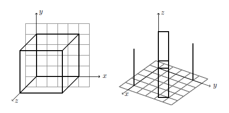
If you look carefully at the rotated diagram, you’ll notice that the rectangles are drawn with the correct beginning and end points, but the overall shape conforms to the original coordinate system of the page.
For More Information
For more information, I recommend you have a look at the package, located at www.ctan.org/pkg/tikz-3dplot.
About the Author:Jeff Hein is the author of the tikz-3dplot package. He maintains a blog for this package on tikz3dplot.wordpress.com.